SQL 2014 Cardinality Estimator: Why You Should Care – Part 2

In the previous post I talked about how query optimization works, the role the Cardinality Estimator (CE) plays, and why you should care. Today I am going to break down some of the details about the differences between the old and new CE, as well as show some examples and scenarios.

What’s New in the SQL 2014 Cardinality Estimator

The CE has remained the same from SQL Server 7.0 through SQL Server 2012. Over the years the SQL Server team has tried to enhance the CE through the use of hotfixes or QFEs through the use of trace flags (so as not to break anything). I like how Juergen Thomas from Microsoft explains in this post:

However to state it pretty clearly as well, it was NOT a goal to avoid any regressions compared to the existing CE. The new SQL Server 2014 CE is NOT integrated following the principals of QFEs. This means our expectation is that the new SQL Server 2014 CE will create better plans for many queries, especially complex queries, but will also result in worse plans for some queries than the old CE resulted in. To define what we mean by better or worse plans, better plans have lower query latency and/or less pages read and worse plans have higher query latency and/or more pages read.

So, there you go. For years we have heard that the product team would never, ever want to introduce something that would break an existing application. But with the new CE changes you can see that mindset was put aside. There was simply no way to update the CE and guarantee that existing code and design would perform as well. Microsoft needed to make a hard choice here, and I’m glad they did. By doing so they help push (and pull) all of us forward. Prior to SQL Server 2014 the legacy CE worked on a set of assumptions:

1. Uniformity – That the data within the logical set was uniformly distributed (in the absence of statistical information).
2. Independence – That the attributes in the entities are independent from each other. In other words, column1 is in no way related to column2.
3. Containment – That two attributes which “might be the same” are treated as the same. In other words, when you join two tables an assumption is made that the distinct values from one table exist in the other.
4. Inclusion – That when an attribute is compared to a constant there is always a match.

The new CE has modified these assumptions, updating them slightly to account for what they call “modern workloads”, a fancy was of saying “stuff we’ve seen since SQL Server 7.0 came out”. As a result of modifying these base assumptions the new CE arrives at different estimates. Which CE is better? It will depend upon your statistics, data distribution, and data design. I’m guessing that this is not the first time you have heard such things with regards to performance. So how can you tell if the new CE is performing better for you? That part is surprisingly easy.

Comparing Old and New CEs

When using SQL Server 2014 you will have the option of using either the legacy or new CE. One way to use the legacy CE is to set your database to an earlier compatibility level. I can take a database created on my SQL Server 2014 instance and set the compatibility level to SQL Server 2012 with the following command:

ALTER DATABASE [db_name] SET COMPATIBILITY_LEVEL = 110
GO

Once complete, all queries in that database will use the legacy CE. I could also leave the database with a compatibility level of 120 (hence, a SQL Server 2014 database) and all queries would use the new CE. If you are wondering what the implications are for toggling between compatibility modes for your databases in SQL Server, go read this TechNet article. You don’t want to just start flipping modes without understanding some of the details in that article.

Ideally, what we need is a way for us to easily toggle between the two CEs, and we can do that by using the following query hints:

OPTION (querytraceon 9481) -- If database in compat level 120, this hint will revert to 2012 CE
OPTION (querytraceon 2312) -- If database in compat level 110, this hint will use new 2014 CE

You can read more details about these hints and compatibility modes here. They are handy to have when you want to verify if the new CE is performing as well (or not) as the legacy CE. I like to keep my database at a compatibility level of 120 and use the 9481 query hint to see the legacy behavior. But that’s just me, you should do what is right for you. With that in mind, we can look at some common scenarios where you are going to see differences between the legacy and new CEs.

Example 1 – Independence

I believe the most significant change with the new CE has to do with the second assumption (Independence). In the legacy CE, which was written against old designs and workloads, the assumption was clear that columns inside of a table had no relation. But we know that is not very practical these days. We can find many cases where values in different columns within one table are not independent of each other. Think about a car brand like Toyota, Volkswagen, Ford, Mercedes, etc. being represented in one column and the type like Corolla, Jetta, Focus or E-Class being represented in another column of a table. It immediately becomes clear that certain combinations can’t happen since Volkswagen is not producing a car named ‘Corolla’.

We can see a quick example of this inside of the AdventureWorksDW2012 database (you can download a copy for yourself here). Once you restore the AdventureWorksDW2012 database to your SQL Server 2014 instance it will be in a compatibility mode of 110, so be mindful of that. I’ve updated mine to be compatibility level 120 and will run the following statement and grab the actual execution plan:

SELECT * 
FROM FactInternetSales
Where currencyKey = 98
AND SalesTerritoryKey = 10
OPTION (QUERYTRACEON 9481) -- revert to 2012 CE

You can see the estimated numbers of rows (just over 770) and actual number of rows (6701) displayed in the properties of the clustered index scan operator: 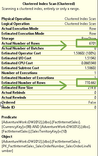Now, let’s run this again, but without the query hint (i.e., using the new CE):

SELECT * 
FROM FactInternetSales
Where currencyKey = 98
AND SalesTerritoryKey = 10

And the properties this time reveal a different number of estimated rows (2279): 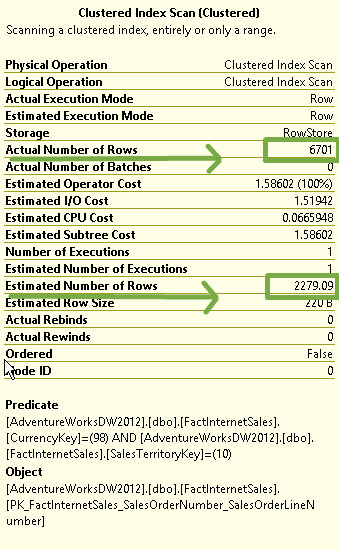So, why the change? One word: math. Since the legacy CE assumes independence of the predicates it uses the following formula:

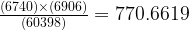
In this case, with 6,740 rows, we end up with:

The new CE assumes some correlation between the predicates and uses different approach called the “exponential backoff algorithm”, which becomes:

In this case, the math works out to be this:

What this means for users of SQL Server 2014 is simple: If you have data with correlating predicates the new CE is likely to give you a better estimate and therefore a better plan. However, if your predicates have no correlation, you may find the legacy CE to provide a better estimate.

One thing to note here is that for this scenario of non-correlated predicates the new CE is likely to result in a slight over-estimation. I am finding it to be the case that I often see the new CE ending up with an overestimation as a result of the new assumptions. In my opinion, I think this is better for the end user. I’d rather have an overestimation as opposed to underestimating, as the underestimation usually results in the optimizer choosing something like a nested loop join when a merge or hash join would have been a better choice. [That’s my long winded way of saying “I’d prefer to use the new CE until my data forces me to revert to the legacy CE for some query”.]

Example 2 – Ascending Keys

Another significant change with the new CE has to do with the “ascending key problem“. You can click the link for more details on the issue itself, I won’t detail them here again. But the new CE handles this scenario better, as it will assume that rows do exist, which results in a better estimate and often a better plan choice. We can see this with a quick example (provided to me by Yi Fang from the SQL Server product team) against the FactCurrencyRate table in the AdventureWorks2012 database.

First, we add some extra columns at the end of the FactCurrencyRate table, so they will fall outside the range of the currently available statistical histogram (i.e., the classic ascending key issue).

-- add 10 rows with DateKey = 20121201
insert into FactCurrencyRate values(3, 20101201, 1, 1, '2010-12-01 00:00:00.000')
insert into FactCurrencyRate values(6, 20101201, 1, 1, '2010-12-01 00:00:00.000')
insert into FactCurrencyRate values(14, 20101201, 1, 1, '2010-12-01 00:00:00.000')
insert into FactCurrencyRate values(16, 20101201, 1, 1, '2010-12-01 00:00:00.000')
insert into FactCurrencyRate values(19, 20101201, 1, 1, '2010-12-01 00:00:00.000')
insert into FactCurrencyRate values(29, 20101201, 1, 1, '2010-12-01 00:00:00.000')
insert into FactCurrencyRate values(36, 20101201, 1, 1, '2010-12-01 00:00:00.000')
insert into FactCurrencyRate values(39, 20101201, 1, 1, '2010-12-01 00:00:00.000')
insert into FactCurrencyRate values(61, 20101201, 1, 1, '2010-12-01 00:00:00.000')
insert into FactCurrencyRate values(85, 20101201, 1, 1, '2010-12-01 00:00:00.000')

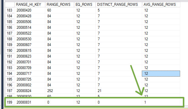
The inserted rows are few enough to not trigger an automatic update of statistics. As a result, the DBCC SHOW_STATISTICS reveals what the end of the histogram looks like. Note the value for the AVG_RANGE_ROWS column:

Now let’s look at a simple query against the range of values that we inserted. This is a fairly common data design and access pattern: inserting data based upon a current date, and that date is then used for queries such as this:

SELECT * 
FROM FactCurrencyRate 
WHERE DateKey = 20101201
OPTION (QUERYTRACEON 9481) -- revert to 2012 CE

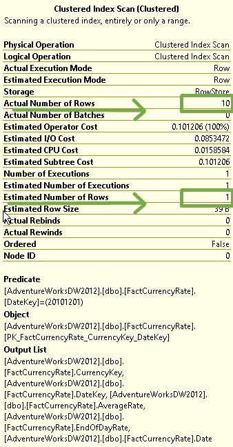
The legacy CE will always return an estimate of 1 row, which is exactly the AVG_RANGE_ROWS value. Essentially, to the legacy CE, we are looking for a range of values for which no statistics exist. You can see this reflected in the properties:

Now let’s look at the new CE, by using the same code without the query hint:

SELECT * 
FROM FactCurrencyRate 
WHERE DateKey = 20101201

Looking at the properties again we can see the estimate has changed:

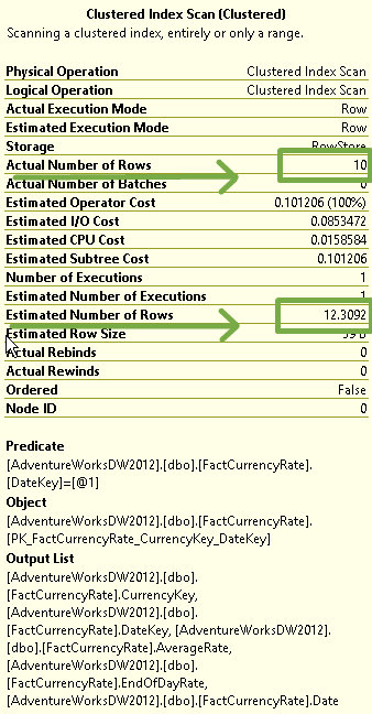
The new CE assumes that some rows exist (otherwise, why would you be searching for them, right?) and therefore bases the estimation upon the average data distribution by taking the cardinality of the table (14,254 rows) and multiplies that by the “All density” value returned in DBCC SHOW_STATISTICS (in this case, that is 0.0008635579). Some quick math shows 14,254 * 0.0008635579 to be equal to 12.30915, which we see displayed as rounded to 12.3092. It’s worth noting that this is the estimate for any values not in the statistics histogram. In this case we have another overestimation, but only because I chose to insert 10 rows. I could have inserted 100 rows and we would have seen the estimate remain at 12.3092.  While this method is far from perfect, I believe it to be better than the legacy estimate of 1.

Example 3 – Containment

Lastly, another important change has to do with the containment assumption. The legacy CE would use a method called “simple containment”, and the new CE uses a method called “base containment”. What the difference you may ask? Great question, let’s take a look using an example from the wonderful whitepaper “Optimizing Your Query Plans with the SQL Server 2014 Cardinality Estimator” written by Joe Sack (blog | @josephsack).

Using a copy of AdventureWorks set to compatibility mode 120, we will run the following query:

SELECT [od].[SalesOrderID], [od].[SalesOrderDetailID]
FROM Sales.[SalesOrderDetail] AS [od]
INNER JOIN Production.[Product] AS [p] 
 ON [od].[ProductID] = [p].[ProductID]
WHERE [p].[Color] = 'Red' AND
[od].[ModifiedDate] = '2008-06-29 00:00:00.000'
OPTION (QUERYTRACEON 9481) -- revert to 2012 CE

The query itself is nothing special, it has a join filter (ProductID) as well as two non-join filter predicates (Color, ModifiedDate), one predicate from each table. This is a fairly common query and we can see the resulting estimate inside the Hash Match operator as follows:

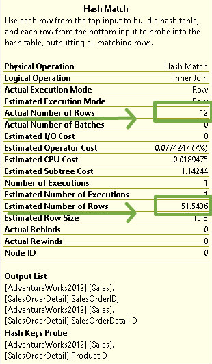
Why 51 rows? The legacy CE assumes that there is likely some level of correlation between predicates. This is called “simple containment” and as a result the legacy CE believes that there must exist some rows that satisfy both. In other words, that sales orders modified on June 28th must also have been for some red colored products.

Let’s run the same code but for the new CE:

SELECT [od].[SalesOrderID], [od].[SalesOrderDetailID]
FROM Sales.[SalesOrderDetail] AS [od]
INNER JOIN Production.[Product] AS [p] 
 ON [od].[ProductID] = [p].[ProductID]
WHERE [p].[Color] = 'Red' AND
[od].[ModifiedDate] = '2008-06-29 00:00:00.000'

This time the Hash Match operator shows a different estimate:

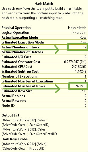
The new CE method of “base containment” does not assume that the predicates from different tables are correlated. It uses estimates from the base tables first, which results in an estimate here that is closer to the actual number of rows.

Summary

There is no question in my mind that the new CE in SQL Server 2014 is the most significant (and overlooked) new feature available. The examples above are trivial in nature, I used them so that you could see the new CE in action. The bigger takeaway I want for you to have from my post today (and yesterday) is to understand how to identify scenarios where the new CE is likely to help (or hurt) your performance and how to quickly verify the differences between the legacy CE and the new CE for any query. While the new CE is likely going to be better in a majority of cases, there will always be some cases where the legacy CE will be a better choice.

I suspect that many people will migrate to SQL 2014 and test their workloads and not even realize the gains just from the new CE alone. Users will probably think that the gains are the result of something else, like newer hardware, more RAM, or faster CPU. I’m hopeful that people will think about baselining performance for their queries by running tests against both the legacy and new CEs, just to verify where the performance gains are really happening.

Or perhaps you want to spend all that money on hardware instead?