SQL 2014 Cardinality Estimator: Why You Should Care

This is the first of two posts on the new Cardinality Estimator in SQL Server 2014. 

SQL Server 2014 comes with a lot of shiny things. Hekaton (or as Microsoft Marketing likes to call it, In-Memory OLTP), updateable Columnstore indexes, and buffer pool extensions are some of the more common enhancements. All of those new features are there to improve performance. Yet there is one thing even more important than all other new things combined: the new Cardinality Estimator (CE).

SQL Server 2014 introduces a brand new CE, and it is the first update to the CE since SQL Server 7.0. Just think about that for a minute…the CE had remained unchanged for almost 20 years! It was originally written for a different era, for different workloads, and for a different average database design. About time they gave it a makeover!

But whenever I talk to people about the new CE they all seem to have a common question. “Why should I care about this?”

I’ll tell you why. But first, let’s take a step backwards and make sure everyone understands the big picture, starting with how SQL Server builds a query plan.

How SQL Builds a Query Plan

This is how most people interact with SQL Server:

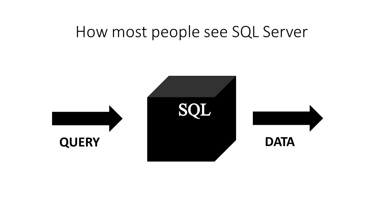
It is a black box, a virtual unknown. For most people in the corporate world the idea of hosted email, virtual machines, or a querying a data warehouse is all the same: it’s magic. It just works.

The reality is that SQL Server has a lot going on under the hood. It is powered by the SQL Operating System (SQLOS). That means it’s an operating system on top of an operating system (i.e., Windows Server), and it looks something like this:

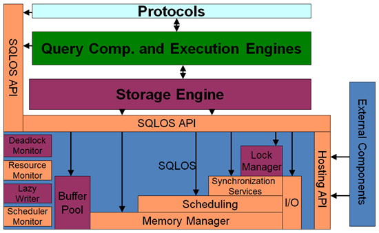
That’s a lot of moving parts, and lots of places for performance tuning and optimization. For this post we are going to focus on the area in green, the query compilation and execution engines, which are not part of the SQLOS but are arguably more critical than everything listed underneath.

Now, when a connection is made to SQL Server it is assigned a session ID (commonly called a SPID). After the connection is made, and a SPID assigned, a request can be made to retrieve data from SQL Server (we often refer to such a request as a “query”). SQL Server has 4 steps to process each query request:

1. Parsing – This is a syntax check, looking for things like reserved keywords.
2. Binding – Also known as “normalization” in SQL 2000, this is now called the algebrizer. It does name resolution and handles aggregates and grouping to form a “query tree”.
3. Optimization – This step takes the query tree and sets about to find a “good enough” plan (i.e., one with the lowest cost). Optimization is cost based and this is the place where statistics and indexes matter most.
4. Execution – Once the plan is found, this is physical retrieval of data from disk and memory.

The first 3 steps are done inside what is known as the Relational Engine, building the logical execution plan. Step four is when calls are made to the Storage Engine to retrieve the data. We are most interested on step 3, Optimization, and what that means.

Finding a “good enough” plan

The primary goal for the Query Optimizer (QO) is to take the query tree that was produced after the Binding phase and to use that to find a “good enough” plan. Why do we say “good enough”? Because there could be thousands or millions of possible plan options and we don’t want SQL Server spending more time than necessary. Thus the concept of “good enough” comes about using a cost-based estimation process.

The cost-based estimates are an abstraction; they don’t relate to anything except other estimates. In other words, they have no unit of value. You can’t say that a plan with lower cost will consume less CPU than another, for example.

The exact details of the query optimizer are unknown, and with good reason. But we don’t need to know the finer details hidden inside of the source code. What we do need is an understanding of the bigger picture on the tasks being done. Paul White (blog | @sql_kiwi) has a great series of blog posts that go into much more detail and if you are interested you can find those posts here. But a summary of the current optimization details provided by the SQL Server team looks something like this:

1. Does plan already exist in cache? If no, then continue to step 2.
2. Is this a trivial plan? If no, then continue.
3. Apply simplification.
4. Is this plan cheap enough? If no, then continue.
5. Start cost-based optimization:
   1. Explore basic rules, compare join operations.
   2. Does plan have a cost of less than 0.2? If no, then continue.
   3. Explore more rules, alternate join ordering. If the best plan is less than 1.0, use that plan. If not, but MAXDOP is > 0 and this is an SMP system and the min cost > cost for parallelism, then use a parallel plan. Compare the cost of parallel plan to best serial plan and pass the cheaper of the plans along.
6. Explore all options, but opt for the cheapest plan after a limited number of explorations.

We are fairly deep inside the rabbit hole at this point. We started inside the green box above, then dove deeper into the query optimization phase, and now we must prepare to go even deeper.

Why the Cardinality Estimator matters SO MUCH!

Stop and think about where we are. Look again at the picture of the SQLOS above. We are deep inside that tiny green box right now.

Now stop and think about a molecule of DNA, which exists in every one of your cells. Your DNA is arguably the most important piece of your physical being, yet it is not something that is easily seen, or understood (except to a very few).

The query optimizer is a lot like our DNA. It seems small, but the role it plays is large. Neither the query optimizer nor your DNA are trivial pieces of code, either.

So when an end user submits a query, the database engine has to do a lot of work to return a result. In order to build a plan, it has to do cost-based optimization. The optimizer relies on the CE to return an accurate estimate of the number of rows a query requires to be satisfied from each table (or index) and uses that information to develop the cost estimates for each step. That’s right, for each operator you see inside of an execution plan there is an estimate of the number of rows, and that estimate is a result of the CE inside of the query optimizer.

The CE itself relies on statistics being up to date in order to get an accurate estimate of row counts. Statistics are metadata objects that help the CE to understand the data distribution inside of each table and index. If statistics are missing, incorrect, or invalid (remember, for EACH operator this is needed) then you are likely to result in a less than optimal plan.

So, good performance is dependent upon accurate statistics. In a way you can consider statistics to be the most important piece of metadata for your database!

Summary

While all those other new features in SQL Server 2014 are nice and shiny, the new CE may have a larger impact on query performance. The old CE model was based upon assumptions for a different era of database development and workloads. The new CE model has modified these assumptions, resulting in (often) improved estimates that lead to better query plans. I said “often” because there are times when the new CE model may not be as good as the legacy CE.

And that’s why you should care about the changes made to the SQL 2014 Cardinality Estimator. You are going to need to know if the new CE is outperforming the legacy CE, or not. So how will you know?

Come back tomorrow and we will look at some specific examples of the new CE in action and how to compare it to the legacy CE.